Importance Sampling Explained End-to-End
Importance sampling is a useful technique when it’s infeasible for us to sample from the real distribution p, when we want to reduce variance of the current Monte Carlo estimator, or when we only know p up to a multiplicative constant.
I found it confusing when I first learned about importance sampling because it applies to so many different scenarios and there are few resources online that walk us through the end-to-end derivation and reasoning process.
In this post, I will try my best to provide such an explanation, starting from the Monte Carlo Methods and ending with an example walk-through.
Monte Carlo Methods
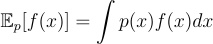
Calculating expectation is an important task in machine learning. Mathematically, given an random variable x with probability density p(x), the expectation of a function of interest f(x) is computed as:
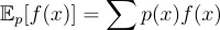
At a high level, expectation can be understood as the probability weighted average of f(x) over the entire space where x lives. When x is discrete, it becomes:
However, when x has high dimension, its probability space becomes exponentially large, making it infeasible to directly calculate the expectation using the integral above. Monte Carlo Methods address this problem by sampling from the probability distribution of x and estimating the expectation from the samples using this formula:
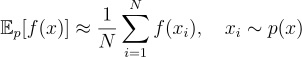
It turns out that this estimation approaches the real expectation as N is large enough.
Bias and Variance of an Estimator
According to Wikipedia, “an estimator is a rule for calculating an estimate of a given quantity based on observed data”. Hence, the process of running the Monte Carlo method yields an estimator for the expectation.
It is important to distinguish between an estimator and a trial of the Monte Carlo method. We can think of an estimator as the aggregate result from running multiple trials of the Monte Carlo method. Due to the randomness in the sampling step, every time we run through the two-step process of sampling and estimating, we produce a slightly different estimation, which we call s, for the expectation. And the estimations themselves have a distribution, which has its own expectation and variance.
The Central Limit Theorem (CLT) states that
“…for independent and identically distributed random variables, the sampling distribution of the standardized sample mean tends towards the standard normal distribution even if the original variables themselves are not normally distributed” - Wikipedia
Translating that into our example, we can say that when N is large enough, the distribution of s is a normal distribution even though p(x) is not normally distributed.
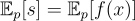
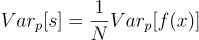
Since Monte Carlo Method generates unbiased estimator for the expectation of a distribution, the expectation and variance of the estimator are computed as follows:
Importance Sampling (IS)
How does IS work?
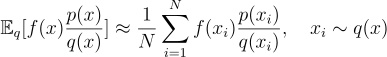
Importance sampling introduces a new distribution q(x), allowing us to get a potentially better estimation of the expectation f(x). Specifically, we can rewrite the expectation formula as follows:

The equation went through the following procedures:
- The integral is multiplied by q(x)/q(x), which is equal to 1 and doesn’t break anything. The only requirement is that we need to have q(x)>0 whenever p(x) is nonzero. This is because if q(x) is zero when p(x) is nonzero, the equation will not hold as some values of x will be missing from the integral.
- Then, we reorder the terms and group f(x)(p(x)/q(x)) as the new function of interest whose expectation we are computing. This allows us to sample from a different distribution q(x) and still get an estimation of the same value - i.e. the expectation of f(x) over p(x) - as before.
Why does IS help?
In the simple term, IS helps because it 1) yields an unbiased estimator and 2) helps lower the variance of the estimator.
Say we use IS and estimate the expectation below:
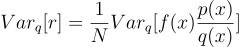
We can compute the expectation and variance of the new estimator r as follows:
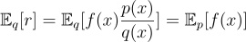
We see that the new estimator r is still an unbiased estimator for the expectation of f(x) since the expectation of r is equal to the value being estimated.
Now that we have an unbiased estimator, let’s look at the variance. In reality, we might not be able to run the Monte Carlo method a large number of times due to cost constraint. Hence, a lower variance for the estimator indicates better quality. We can pick q(x) such that it results in lower variance; that is,
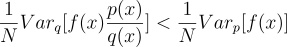
To achieve this, we want q(x) to be large where |p(x)f(x)| is high.
To understand why such q(x) helps reduce the variance, think about a case where f(x) has very uneven distribution while p(x) is a uniform distribution. Also assume that we have a very limited budget and it’s infeasible for us to sample a large amount of examples or run many Monte Carlo trials.
As we see in the left picture, f(x) has a very small region that contributes the most to the expectation. When we cannot sample a large amount from p(x), it’s likely that we miss that small “important” region of f(x), resulting in a bad estimation.
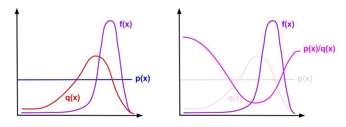
If we pick q(x) such that it allows us to sample from the “important” region with higher probability, we see that the resulting ratio p(x)/q(x) that we multiply f(x) will effectively unweight the “important” regions that we put a higher probability into. This unweighting ratio is what makes the IS estimator unbiased and lowers the variance.
Example
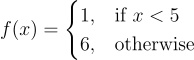
To see how IS reduces variance, let’s look at an example with a discrete random variable X that can take on integer values in range [1,5]. Say p(X) is uniform over all values of X, so we have p(x) = 1/5.
Let’s define the function of interest f(x) as follows:
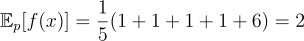
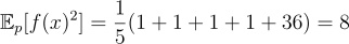
We can compute the expectation and variance of the Monte Carlo estimator over p(x) as follows:

Now say we have a new distribution q(x) defined as follows:
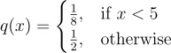
Now, we can compute the expectation and variance of our estimator as follows:
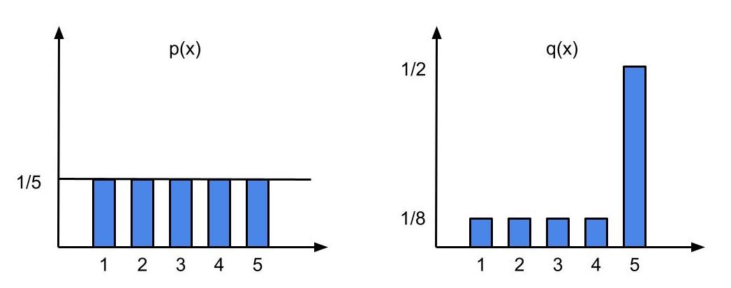
We see that the variance given by the IS estimator is much lower than the one given by the uniform estimator.
References
I hope you enjoyed this article! Connect with me on LinkedIn if you are also interested in AI, ML, databases, and more.